


By Mahavir Bhattacharya
TL;DR:
This weblog introduces retrospective simulation, impressed by Taleb’s “Fooled by Randomness,” to simulate 1,000 alternate historic value paths utilizing a non-parametric Brownian bridge technique. Utilizing SENSEX information (2000–2020) as in-sample information, the writer optimises an EMA crossover technique throughout the in-sample information first, after which applies it to the out-of-sample information utilizing the optimum parameters obtained from the in-sample backtest. Whereas the technique outperforms the buy-and-hold strategy in in-sample testing, it considerably underperforms in out-of-sample testing (2020–2025), highlighting the danger of overfitting to a single realised path. The writer then runs the backtest throughout all simulated paths to determine essentially the most regularly profitable SEMA-LEMA parameter mixtures.
The writer additionally calculates VaR and CVaR utilizing over 5 million simulated returns and compares return extremes and distributional traits, revealing heavy tails and excessive kurtosis. This framework permits extra sturdy technique validation by evaluating how methods would possibly carry out throughout a number of believable market situations.
Introduction
In “Fooled by Randomness”, Taleb says at one place, “At first, after I knew near nothing (that’s, even lower than right this moment), I questioned whether or not the time sequence reflecting the exercise of individuals now useless or retired ought to matter for predicting the long run.”
This acquired me considering. We regularly run simulations for the possible paths a time sequence can take sooner or later. Nevertheless, the premise for these simulations relies on historic information. Given the stochastic nature of asset costs (learn extra), the realised value path had the selection of an infinite variety of paths it might have taken, however it traversed via solely a kind of infinite potentialities. And I believed to myself, why not simulate these alternate paths?
In widespread observe, this strategy is known as bootstrap historic simulation. I selected to confer with it as retrospective simulation, as a extra intuitive counterpart to the phrases ‘look-ahead’ and ‘walk-forward’ used within the context of simulating the long run.
Article map
Right here’s a top level view of how this text is laid out:
Information Obtain
We import the mandatory libraries and obtain the day by day information of the SENSEX index, a broad market index primarily based on the Bombay Inventory Alternate of India.
I’ve downloaded the info from January 2000 to November 2020 because the in-sample information, and from December 2020 to April 2025 because the out-of-sample information. We might have put in a spot (an embargo) between the in-sample and out-of-sample information to minimise, if not remove, information leakage (learn extra). In our case, there’s no direct information leakage. Nevertheless, since inventory ranges (costs) are identified to bear autocorrelation, like we noticed above, the SENSEX index on the primary buying and selling day of December 2020 can be extremely correlated with its stage on the final buying and selling day of November 2020.
Thus, after we prepare our mannequin on information that features the final buying and selling day of November 2020, it extracts info from that day’s stage and makes use of it to get educated. Since our testing dataset is from the primary buying and selling day of December 2020, some residual info from the coaching dataset is current within the testing dataset.
As an extension, the coaching set comprises some info that can be current within the testing dataset. Nevertheless, this info will diminish over time and finally change into insignificant. Having mentioned that, I didn’t preserve a spot between the in-sample and out-of-sample datasets in order that we will concentrate on understanding the core idea of this text.
You need to use any yfinance ticker to obtain information for an asset of your liking. You may also alter the dates to fit your wants.
Retrospective Simulation utilizing Brownian Bridge
The subsequent half is the principle crux of this weblog. That is the place I simulate the potential paths the asset might have taken from January 2000 to November 2020. I’ve simulated 1000 paths. You possibly can modify it to make it 100 or 10000, as you want. The upper the worth, the better our confidence within the outcomes, however there’s a tradeoff in computational time. I’ve simulated solely the closing costs. I stored the first-day and last-day costs the identical because the realised ones, and simulated the in-between costs.
Maintaining the value mounted on the primary day is sensible. However the final day? If the costs are to comply with a random stroll (learn extra), the closing value ranges of most, if not all, paths needs to be totally different, isn’t it? However I made an assumption right here. Given the environment friendly market speculation, the index would have a good value by the tip of November 2020, and after shifting on its capricious course, it might converge again to this honest value.
Why solely November 2020?
Was the extent of the index at its fairest value at the moment? No approach of understanding. Nevertheless, one date is nearly as good as some other, and we have to work with a particular date, so I selected this one.
One other consideration right here is on what foundation we permit the simulated paths to meander. Ought to it’s parametric, the place we assume the time sequence to comply with a particular distribution, or non-parametric, the place we don’t make any such assumption? I selected the latter. The monetary literature discusses costs (and their returns) as belonging roughly to sure underlying distributions. Nevertheless, with regards to outlier occasions, equivalent to extremely unstable value jumps, these assumptions start to interrupt down, and it’s these occasions {that a} quant (dealer, portfolio supervisor, investor, analyst, or researcher) needs to be ready for.
For the non-parametric strategy, I’ve modified the Brownian bridge strategy. In a pure Brownian bridge strategy, the returns are assumed to comply with a Gaussian distribution, which once more turns into considerably parametric (learn extra). Nevertheless, in our strategy, we calculate the realized returns from the in-sample closing costs and use these returns as a pattern for the simulation generator to select from. We’re utilizing bootstrapping with substitute (learn extra), which signifies that the realized returns aren’t simply being shuffled; some values could also be repeated, whereas some might not be used in any respect. If the values are merely shuffled, all simulated paths would land on the final closing value of the in-sample information. How can we be sure that the simulated costs converge to the ultimate shut value of the in-sample information? We’ll use geometric smoothing for that.
One other consideration: since we use the realized returns, we’re priming the simulated paths to resemble the realized path, appropriate? Kind of, but when we have been to generate pseudo-random numbers for these returns, we must make some assumption about their distribution, making the simulation a parametric course of.
Right here’s the code for the simulations:
Be aware that I didn’t use a random seed when producing the simulated paths. I’ll point out the explanation at a later stage.
Let’s plot the simulated paths:

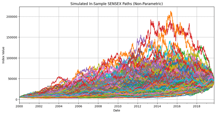
The above graph exhibits that the beginning and ending costs are the identical for all 1,000 simulated paths. We should always word one factor right here. Since we’re working with information from a broad market index, whose ranges depend upon many interlinked macroeconomic variables and elements, it is extremely unlikely that the index would have traversed many of the paths simulated above, given the identical macroeconomic occasions that occurred throughout the simulation interval. We’re making an implicit assumption right here that the desired macroeconomic variables and elements differ in every of the simulated paths, and the interactions between these variables and elements outcome within the simulated ranges that we generate. This holds for some other asset class or asset you resolve to exchange the SENSEX index with, for retrospective simulation functions.
Exponential Shifting Common Crossover Technique Improvement and Backtesting on In-Pattern Information, and Parameter Optimisation
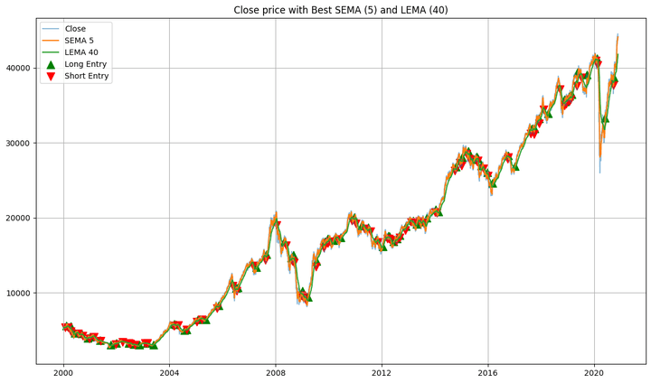
Subsequent, we develop a easy buying and selling technique and conduct a backtest utilizing the in-sample information. The technique is a straightforward exponential shifting common crossover technique, the place we go lengthy when the short-period exponential shifting common (SEMA) of the shut value goes above the long-period exponential shifting common (LEMA), and we go quick when the SEMA crosses the LEMA from above (learn extra).
Via optimisation, we’ll try to search out the perfect SEMA and LEMA mixture that yields the utmost returns. For the SEMA, I exploit lookback intervals of 5, 10, 15, 20, … as much as 100, and for the LEMA, 20, 30, 40, 50, … as much as 300.
The situation is that for any given SEMA and LEMA mixture, the LEMA lookback interval needs to be better than the corresponding SEMA lookback interval. We might carry out backtests on all totally different mixtures of those SEMA and LEMA values and select the one which yields the perfect efficiency.
We’ll plot:
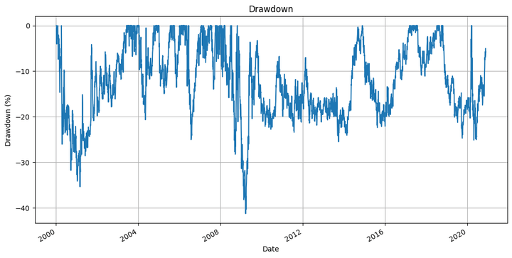
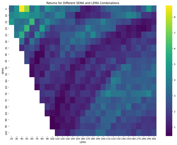
the fairness curve of the technique with the best-performing SEMA and LEMA lookback values, plotted towards the buy-and-hold fairness,the purchase and promote indicators plotted together with the shut costs of the in-sample information and the SEMA and LEMA strains,the underwater plot of the technique, and,a heatmap of the returns for various LEMA and SEMA calculations.
We’ll calculate:
the SEMA and LEMA lookback values for the best-performing mixture,the entire returns of the technique,the utmost drawdown of the technique, and,the Sharpe ratio of the technique.
We will even evaluate the highest 10 SEMA and LEMA mixtures and their respective performances.
Right here’s the code for the entire above:
And listed here are the outputs of the above code:
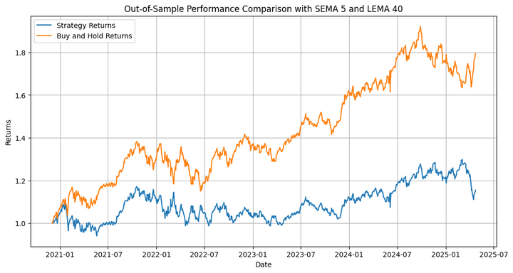
Greatest SEMA: 5, Greatest LEMA: 40

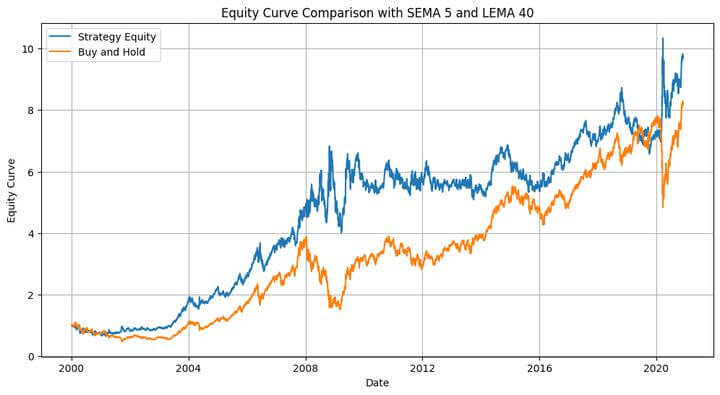

Whole Return: 873.43%
Most Drawdown: -41.28 %
Sharpe Ratio: 0.59


High 10 Parameter Mixtures:
SEMA LEMA Return
2 5 40 8.734340
3 5 50 7.301270
62 15 60 6.021219
89 20 50 5.998316
116 25 40 5.665505
31 10 40 5.183363
92 20 80 5.071913
32 10 50 5.022373
58 15 20 4.959147
27 5 290 4.794400
The heatmap exhibits a gradual change in colour from one adjoining cell to the subsequent. This implies that slight modifications to the EMA values don’t result in drastic modifications within the technique’s efficiency. After all, it might be extra gradual if we have been to cut back the spacing between the SEMA values from 5 to, say, 2, and between the LEMA values from 10 to, say, 3.
The technique outperforms the buy-and-hold technique, as proven within the fairness plot. Excellent news, proper? Be aware right here that this was in-sample backtesting. We ran the optimisation on a given dataset, took some info from it, and utilized it to the identical dataset. It’s like utilizing the costs for the subsequent yr (that are unknown to us now, besides for those who’re time-travelling!) to foretell the costs over the subsequent yr. Nevertheless, we will utilise the data gathered from this dataset to use it to a different dataset. That’s the place we use the out-of-sample information.
Backtesting on Out-of-Pattern Information
Let’s run the backtest on the out-of-sample dataset:
Earlier than we see the outputs of the above codes, let’s checklist what we’re doing right here.
We’re plotting:
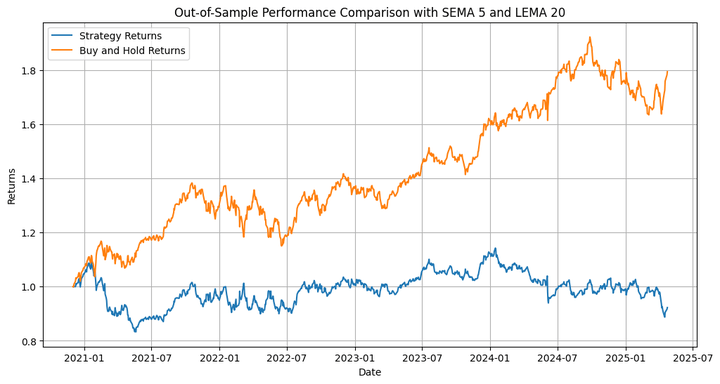
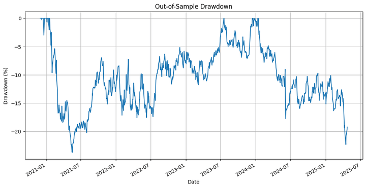
The fairness curve of the technique plotted alongside that of the buy-and-hold, and,The underwater plot of the technique.
We’re calculating:
Technique returns,Purchase-and-hold returns,Technique most drawdown,Technique Sharpe ratio,Purchase-and-hold Sharpe ratio, and,Technique hit ratio.
For the Sharpe ratio calculations, we assume a risk-free fee of return of 0. Listed here are the outputs:
Out-of-Pattern Technique Whole Return: 15.46%
Out-of-Pattern Purchase-and-Maintain Whole Return: 79.41%
Out-of-Pattern Technique Most Drawdown: -15.77 %
Out-of-Pattern Technique Sharpe Ratio: 0.30
Out-of-Pattern Purchase-and-Maintain Sharpe Ratio: 0.56
Out-of-Pattern Hit Ratio: 53.70%


The technique underperforms the underlying by a major margin. However that’s not what we’re primarily desirous about, so far as this weblog is anxious. We have to think about that we ran an optimisation on solely one of many many paths that the costs might have taken throughout the in-sample interval, after which extrapolated that to the out-of-sample backtest. That is the place we use the simulation we carried out in the beginning. Let’s run the backtest on the totally different simulated paths and test the outcomes.
Backtesting on Simulated Paths and Optimising to Extract the Greatest Parameters
This is able to preserve printing the corresponding SEMA and LEMA values for the perfect technique efficiency, and the efficiency itself for the simulated paths:
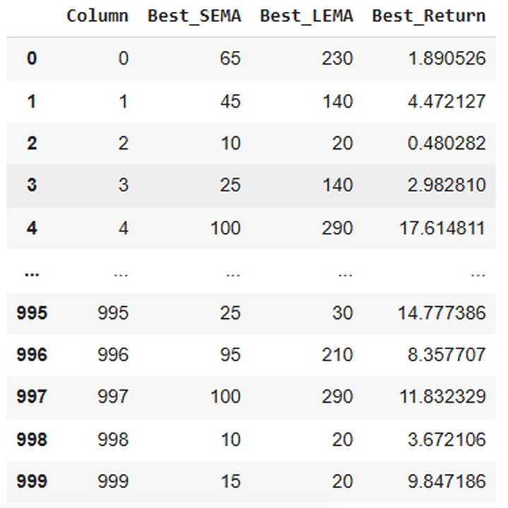
Accomplished optimization for column 0: SEMA=65, LEMA=230, Return=1.8905
Accomplished optimization for column 1: SEMA=45, LEMA=140, Return=4.4721
……………………………………………………………
Accomplished optimization for column 998: SEMA=10, LEMA=20, Return=3.6721
Accomplished optimization for column 999: SEMA=15, LEMA=20, Return=9.8472
Right here’s a snap of the output of this code:

Now, we’ll type the above desk in order that the SEMA and LEMA mixture with the perfect returns for essentially the most paths is on the prime, adopted by the second-best mixture, and so forth.
Let’s test how the desk would look:
Right here’s a snapshot of the output:

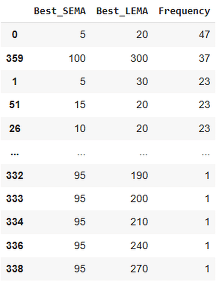
Of the 1000 paths, 47 confirmed the perfect returns with a mixture of SEMA 5 and LEMA 20. Since I didn’t use a random seed whereas producing the simulated paths, you possibly can run the code a number of instances and procure totally different outputs or outcomes. You’ll see that the perfect SEMA and LEMA mixture within the above desk would almost certainly be 5 and 20. The frequencies can change, although.
How do I do know?
As a result of I’ve carried out so, and have gotten the mixture of 5 and 20 within the first place each time (adopted by 100 and 300 within the second place). After all, it’s not that there’s a zero likelihood of getting another mixture within the prime row.
Out-of-Pattern Backtesting utilizing Optimised Parameters primarily based on Simulated Information Backtesting
We’ll extract the SEMA and LEMA look-back mixture from the earlier step that yields the perfect returns for many of the simulated paths. We’ll use a dynamic strategy to automate this choice. Thus, if as an alternative of 5 and 20, we have been to acquire, say, 90 and 250 because the optimum mixture, the identical can be chosen, and the backtest can be carried out utilizing that.
Let’s use this mixture to run an out-of-sample backtest:
Listed here are the outputs:
Out-of-Pattern Technique Whole Return: -7.73%
Out-of-Pattern Purchase-and-Maintain Whole Return: 79.41%
Out-of-Pattern Technique Most Drawdown: -23.70 %
Out-of-Pattern Technique Sharpe Ratio: -0.05
Out-of-Pattern Purchase-and-Maintain Sharpe Ratio: 0.56
Out-of-Pattern Hit Ratio: 52.50%
Dialogue on the Outcomes and the Method
Right here, the technique not solely underperforms the underlying but additionally generates detrimental returns. So what’s the purpose of all this effort that we put in? Let’s word that I employed the shifting common crossover technique to illustrate the applying of retrospective simulation utilizing a modified Brownian bridge. This strategy is extra appropriate for testing advanced methods with a number of circumstances, and machine studying (ML)-based and deep studying (DL)-based methods.
We have now approaches equivalent to walk-forward optimisation and cross-validation to beat the issue of optimising or fine-tuning a method or mannequin on solely one of many many potential traversable paths.
Nevertheless, this strategy of retrospective simulation ensures that you simply don’t need to depend on just one path however can make use of a number of retrospective paths. Nevertheless, since operating an ML-based technique on these simulated paths can be too computationally intensive for many of our readers who don’t have entry to GPUs or TPUs, I selected to work with a easy technique.
Moreover, for those who want to modify the strategy, I’ve included some options on the finish.
Analysis of VaR and C-VaR
Let’s transfer on to the subsequent half. We’ll utilise the retrospective simulation to calculate the worth in danger and the conditional worth in danger (learn extra: 1, 2, 3).
Output:
Worth at Danger – 90%: -0.014976172535594811
Worth at Danger – 95%: -0.022113806787530325
Worth at Danger – 99% -0.04247765359038646
Anticipated Shortfall – 90%: -0.026779592114352924
Anticipated Shortfall – 95%: -0.035320511964199504
Anticipated Shortfall – 99% -0.058565593363193474
Let’s decipher the above output. We first calculated the day by day % returns of all 1000 simulated paths. Each path has 5,155 days of knowledge, which yielded 5,154 returns per path. When multiplied by 1,000 paths, this resulted in 5,154,000 values of day by day returns. We used all these values and located the bottom ninetieth, ninety fifth, and 99th percentile values, respectively.
From the above output, for instance, we will say with 95% certainty that if the long run costs comply with paths much like these simulated paths, the utmost drawdown that we will face on any given day can be 2.21%. The anticipated drawdown can be 3.53% if that stage will get breached.
Let’s speak concerning the extremes now. Let’s examine the utmost and minimal day by day returns of the simulated paths and the realised in-sample path.
Realized Lowest Each day Return: -0.1315258002691394
Realized Highest Each day Return: 0.17339334818061447
The utmost values from each approaches are shut, at round 17.4%. Similar for the minimal values, at round -13.2%. This makes a case for utilizing this strategy in monetary modelling.
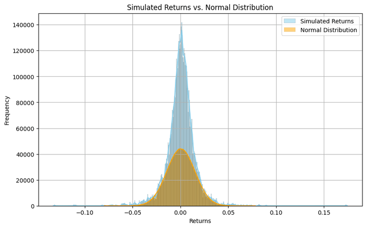
Distribution of Simulated Information
Let’s see how the simulated returns are distributed and examine them visually to a standard distribution. We’ll additionally calculate the skewness and the kurtosis.

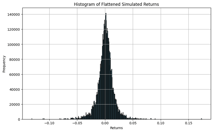
Skewness: -0.11595652411010503
Kurtosis: 9.597364213156881
The argument ‘kde’, when set to ‘True’, smooths the histogram curve, as proven within the above plot. Additionally, in order for you a extra granular (coarse) visible of the distribution, you possibly can enhance (cut back) the worth within the ‘bins’ argument.
Although the histogram resembles a bell curve, it’s removed from a standard distribution. It displays heavy kurtosis, which means there are important probabilities of discovering returns which might be many commonplace deviations away from the imply. And this isn’t any shock, since that’s how fairness and equity-index returns are inherently.
The place This Method Can Be Most Helpful
Whereas the technique I used right here is easy and illustrative, this retrospective simulation framework comes into its personal when utilized to extra advanced or nuanced methods. It’s helpful in instances the place:
You are testing multi-condition or ML-based fashions that may overfit on a single realized path.You need to stress check a method throughout alternate historic realities—ones that didn’t occur, however very effectively might have.Conventional walk-forward or cross-validation strategies don’t appear to be sufficient, and also you need an added lens to judge generalisability.You are exploring how a method would possibly behave (or may need behaved had the value taken on any alternate value path) underneath excessive market strikes that aren’t current within the precise historic path.
In essence, this technique lets you transition from “what occurred” to “what might have occurred,” a delicate but highly effective shift in perspective.
Recommended Subsequent Steps
In case you discovered this strategy attention-grabbing, listed here are just a few methods you possibly can lengthen it:
Strive extra refined methods: Apply this retrospective simulation to mean-reversion, volatility breakout, or reinforcement learning-based methods.Introduce macro constraints: Anchor the simulations round identified macroeconomic markers or regime modifications to check how methods behave in such environments.Use intermediate anchor factors: As an alternative of simply fixing the beginning and finish costs, attempt anchoring the simulation at quarterly or annual ranges to raised management drift and convergence.Practice ML fashions on simulated paths: In case you’re working with supervised studying or deep studying fashions, prepare them on a number of simulated realities as an alternative of 1.Portfolio-level testing: Use this framework to judge VaR, CVaR, or stress-test a complete portfolio, not only a single technique.
That is just the start—the way you construct on it depends upon your curiosity, computing sources, and the questions you are attempting to reply.
In Abstract
The weblog launched a retrospective simulation framework utilizing a non-parametric Brownian bridge strategy to simulate alternate historic value paths.We employed a easy EMA crossover technique to illustrate how this simulation will be built-in into a conventional backtesting loop.We extracted the perfect SEMA and LEMA mixtures after operating backtests on the simulated in-sample paths, after which used these for backtesting on the out-of-sample information.This simulation technique permits us to check how methods would behave not solely in response to what occurred, but additionally in response to what might have occurred, serving to us keep away from overfitting and uncover sturdy indicators.The identical simulated paths can be utilized to derive distributional insights, equivalent to tail danger (VaR, CVaR) or return extremes, providing a deeper understanding of the technique’s danger profile.
Ceaselessly Requested Questions
1. Curious why we simulate value paths in any respect?Actual market information exhibits just one path the market took, amongst many potential paths. However what if we need to perceive how our technique would behave throughout many believable realities sooner or later, or would have behaved throughout such realities prior to now? That’s why we use simulations.
2. What precisely is a Brownian bridge, and why was it used?A Brownian bridge simulates value actions that begin and finish at particular values, like actual historic costs. This helps guarantee simulated paths are anchored in actuality whereas nonetheless permitting randomness in between. The principle query we ask right here is “What else might have occurred prior to now?”.
3. What number of simulated paths ought to I generate to make this evaluation significant?We used 1000 paths. As talked about within the weblog, when the variety of simulated paths will increase, computation time will increase, however our confidence within the outcomes grows too.
4. Is that this solely for easy methods like shifting averages?In no way. We used the shifting common crossover simply for example. This framework will be (and needs to be) used while you’re testing advanced, ML-based, or multi-condition methods which will overfit to historic information.
5. How do I discover the perfect parameter settings (like SEMA/LEMA)?For every simulated path, we backtested totally different parameter mixtures and recorded the one which gave the very best return. By counting which mixtures carried out greatest throughout most simulations, we recognized the mixture that’s almost certainly to carry out effectively. The thought is to not depend on the mixture that works on only one path.
6. How do I do know which parameter combo to make use of within the markets?The thought is to choose the combo that the majority regularly yielded the perfect outcomes throughout many simulated realities. This helps keep away from overfitting to the only historic path and as an alternative focuses on broader adaptability. The precept right here is to not let our evaluation and backtesting be topic to likelihood or randomness, however slightly to have some statistical significance.
7. What occurs after I discover that “greatest” parameter mixture?We run an out-of-sample backtest utilizing that mixture on information the mannequin hasn’t seen. This assessments whether or not the technique works exterior of the info on which the mannequin is educated.
8. What if the technique fails within the out-of-sample check?That’s okay, and on this instance, it did! The purpose is to not “win” with a fundamental technique, however to point out how simulation and sturdy testing reveal weaknesses earlier than actual cash is concerned. After all, while you backtest an precise alpha-generating technique utilizing this strategy and nonetheless get underperformance within the out-of-sample, it seemingly signifies that the technique isn’t sturdy, and also you’ll have to make modifications to the technique.
9. How can I exploit these simulations to know potential losses?We adopted the strategy of flattening the returns from all simulated paths into one huge distribution and calculating danger metrics like Worth at Danger (VaR) and Conditional VaR (CVaR). These present how dangerous issues can get, and the way typically.
10. What’s the distinction between VaR and CVaR?
VaR tells us the worst anticipated loss at a given confidence stage (e.g., “you’ll lose not more than 2.2% on 95% of days”).CVaR goes a step additional and says, “In case you lose greater than that, right here’s the common of these worst days.”.
11. What did we study from the VaR/CVaR outcomes on this instance?We noticed that 99% of days resulted in losses no worse than ~4.25%. However when losses exceeded that threshold, they averaged ~5.86%. That’s a helpful perception into tail danger. These are the uncommon however extreme occasions that may extremely have an effect on our buying and selling accounts if not accounted for.
12. Are the simulated return extremes practical in comparison with actual markets?Sure, they matched very carefully with the utmost and minimal day by day returns from the true in-sample information. This validates that our simulation isn’t simply random however is grounded in actuality.
13. Do the simulated returns comply with a standard distribution?Not fairly. The returns confirmed excessive kurtosis (fats tails) and slight detrimental skewness, which means excessive strikes (each up and down) are extra widespread than a standard distribution would have. This mirrors actual market behaviour.
14. Why does this matter for danger administration?If our technique assumes regular returns, we’re closely underestimating the likelihood of serious losses. Simulated returns reveal the true nature of market danger, serving to us put together for the sudden.
15. Is that this simply an instructional train, or can I apply this virtually? This strategy is extremely helpful in observe, particularly while you’re working with:
Machine studying fashions which might be vulnerable to overfittingStrategies designed for high-risk environmentsPortfolios the place stress testing and tail danger are crucialRegime-switching or macro-anchored fashions
It helps shift our mindset from “What labored earlier than?” to “What would have labored throughout many alternate market situations?”, and that may be one latent supply of alpha.
Conclusion
Hope you discovered at the least one new factor from this weblog. In that case, do share what it’s within the feedback part beneath and tell us for those who’d prefer to learn or study extra about it. The important thing takeaway from the above dialogue is the significance of performing simulations retrospectively and making use of them to monetary modelling. Apply this strategy to extra advanced methods and share your experiences and findings within the feedback part. Comfortable studying, completely happy buying and selling 🙂
Credit
José Carlos Gonzáles Tanaka and Vivek Krishnamoorthy, thanks in your meticulous suggestions; it helped form this text!
Chainika Thakar, thanks for rendering and publishing this, and making it obtainable to the world, that too in your birthday!
Disclaimer: All investments and buying and selling within the inventory market contain danger. Any resolution to put trades within the monetary markets, together with buying and selling in inventory or choices or different monetary devices is a private resolution that ought to solely be made after thorough analysis, together with a private danger and monetary evaluation and the engagement {of professional} help to the extent you imagine vital. The buying and selling methods or associated info talked about on this article is for informational functions solely.


